Steps 1-6
- Load the R packages we will use
2.Read the data in the files, drug_cos.csv, health_cos.csv in to R and assign to the variables drug_cos and health_cos, respectively
drug_cos  <- read_csv("https://estanny.com/static/week6/drug_cos.csv")
health_cos  <- read_csv("https://estanny.com/static/week6/health_cos.csv")
drug_cos %>% glimpse()
Rows: 104
Columns: 9
$ ticker       <chr> "ZTS", "ZTS", "ZTS", "ZTS", "ZTS", "ZTS", "ZTS…
$ name         <chr> "Zoetis Inc", "Zoetis Inc", "Zoetis Inc", "Zoe…
$ location     <chr> "New Jersey; U.S.A", "New Jersey; U.S.A", "New…
$ ebitdamargin <dbl> 0.149, 0.217, 0.222, 0.238, 0.182, 0.335, 0.36…
$ grossmargin  <dbl> 0.610, 0.640, 0.634, 0.641, 0.635, 0.659, 0.66…
$ netmargin    <dbl> 0.058, 0.101, 0.111, 0.122, 0.071, 0.168, 0.16…
$ ros          <dbl> 0.101, 0.171, 0.176, 0.195, 0.140, 0.286, 0.32…
$ roe          <dbl> 0.069, 0.113, 0.612, 0.465, 0.285, 0.587, 0.48…
$ year         <dbl> 2011, 2012, 2013, 2014, 2015, 2016, 2017, 2018…
health_cos %>% glimpse()
Rows: 464
Columns: 11
$ ticker      <chr> "ZTS", "ZTS", "ZTS", "ZTS", "ZTS", "ZTS", "ZTS"…
$ name        <chr> "Zoetis Inc", "Zoetis Inc", "Zoetis Inc", "Zoet…
$ revenue     <dbl> 4233000000, 4336000000, 4561000000, 4785000000,…
$ gp          <dbl> 2581000000, 2773000000, 2892000000, 3068000000,…
$ rnd         <dbl> 427000000, 409000000, 399000000, 396000000, 364…
$ netincome   <dbl> 245000000, 436000000, 504000000, 583000000, 339…
$ assets      <dbl> 5711000000, 6262000000, 6558000000, 6588000000,…
$ liabilities <dbl> 1975000000, 2221000000, 5596000000, 5251000000,…
$ marketcap   <dbl> NA, NA, 16345223371, 21572007994, 23860348635, …
$ year        <dbl> 2011, 2012, 2013, 2014, 2015, 2016, 2017, 2018,…
$ industry <chr> "Drug Manufacturers - Specialty & Generic", "Dr…- Which variables are the same in both data sets
names_drug  <- drug_cos  %>%  names()
names_health  <- health_cos  %>%  names()
intersect(names_drug, names_health)
[1] "ticker" "name" "year" 5.Select subset of variables to work with
-For drug_cos select (in this order): ticker, year, grossmargin
-Extract observations for 2018
-Assign output to drug_subset
-For health_cos select (in this order): ticker, year, revenue, gp, industry
-Extract observations for 2018
-Assign output to health_subset
drug_subset join with columns in health_subset
drug_subset %>% left_join(health_subset)
# A tibble: 13 x 6
   ticker  year grossmargin   revenue        gp industry
   <chr>  <dbl>       <dbl>     <dbl>     <dbl> <chr>
 1 ZTS     2018       0.672   5.82e 9   3.91e 9 Drug Manufacturers - …
 2 PRGO    2018       0.387   4.73e 9   1.83e 9 Drug Manufacturers - …
 3 PFE     2018       0.79    5.36e10   4.24e10 Drug Manufacturers - …
 4 MYL     2018       0.35    1.14e10   4.00e 9 Drug Manufacturers - …
 5 MRK     2018       0.681   4.23e10   2.88e10 Drug Manufacturers - …
 6 LLY     2018       0.738   2.46e10   1.81e10 Drug Manufacturers - …
 7 JNJ     2018       0.668   8.16e10   5.45e10 Drug Manufacturers - …
 8 GILD    2018       0.781   2.21e10   1.73e10 Drug Manufacturers - …
 9 BMY     2018       0.71    2.26e10   1.60e10 Drug Manufacturers - …
10 BIIB    2018       0.865   1.35e10   1.16e10 Drug Manufacturers - …
11 AMGN    2018       0.827   2.37e10   1.96e10 Drug Manufacturers - …
12 AGN     2018       0.861   1.58e10   1.36e10 Drug Manufacturers - …
13 ABBV 2018 0.764 3.28e10 2.50e10 Drug Manufacturers - …Question:join_ticker
- Start with
drug_cosExtract observations for the ticker JNJ fromdrug_cosAssign output to the variabledrug_cos_subset
drug_cos_subset <- drug_cos %>%
  filter(ticker == "JNJ")
-Display drug_cos_subset
drug_cos_subset
# A tibble: 8 x 9
  ticker name  location ebitdamargin grossmargin netmargin   ros   roe
  <chr>  <chr> <chr>           <dbl>       <dbl>     <dbl> <dbl> <dbl>
1 JNJ    John… New Jer…        0.247       0.687     0.149 0.199 0.161
2 JNJ    John… New Jer…        0.272       0.678     0.161 0.218 0.173
3 JNJ    John… New Jer…        0.281       0.687     0.194 0.224 0.197
4 JNJ    John… New Jer…        0.336       0.694     0.22  0.284 0.217
5 JNJ    John… New Jer…        0.335       0.693     0.22  0.282 0.219
6 JNJ    John… New Jer…        0.338       0.697     0.23  0.286 0.229
7 JNJ    John… New Jer…        0.317       0.667     0.017 0.243 0.019
8 JNJ    John… New Jer…        0.318       0.668     0.188 0.233 0.244
# … with 1 more variable: year <dbl>
-Use left_join to combine the rows and columns of drug_cos_subset with the columns of health_cos
-Assign the output to combo_df
 combo_df <- drug_cos_subset  %>%
   left_join(health_cos)
-Display
combo_df
combo_df
# A tibble: 8 x 17
  ticker name  location ebitdamargin grossmargin netmargin   ros   roe
  <chr>  <chr> <chr>           <dbl>       <dbl>     <dbl> <dbl> <dbl>
1 JNJ    John… New Jer…        0.247       0.687     0.149 0.199 0.161
2 JNJ    John… New Jer…        0.272       0.678     0.161 0.218 0.173
3 JNJ    John… New Jer…        0.281       0.687     0.194 0.224 0.197
4 JNJ    John… New Jer…        0.336       0.694     0.22  0.284 0.217
5 JNJ    John… New Jer…        0.335       0.693     0.22  0.282 0.219
6 JNJ    John… New Jer…        0.338       0.697     0.23  0.286 0.229
7 JNJ    John… New Jer…        0.317       0.667     0.017 0.243 0.019
8 JNJ    John… New Jer…        0.318       0.668     0.188 0.233 0.244
# … with 9 more variables: year <dbl>, revenue <dbl>, gp <dbl>,
#   rnd <dbl>, netincome <dbl>, assets <dbl>, liabilities <dbl>,
#   marketcap <dbl>, industry <chr>
-Note: the variables ticker, name, location and industry are the same for all the observations
-Assign the company name to co_name
co_name<- combo_df  %>%
  distinct(name) %>%
  pull()
-Assign the company location to co_location
co_location  <- combo_df  %>%
  distinct(location)  %>%
  pull()
-Assign the industry to
co_industry group
co_industry  <- combo_df  %>%
  distinct(industry)  %>%
  pull()
Put the r inline commands used in the blanks below. When you knit the document the results of the commands will be displayed in your text.
The company Johnson & Johnson is located in New Jersey;U.S.A and is a member of the Drug Manufacturers industry group.
-Start with combo_df
-Select variables (in this order): year, grossmargin, netmargin, revenue, gp, netincome
-Assign the output to combo_df_subset
combo_df_subset  <- combo_df  %>%
  select(year, grossmargin, netmargin,
  revenue, gp, netincome)
-Display
combo_df_subset
combo_df_subset
# A tibble: 8 x 6
   year grossmargin netmargin     revenue          gp   netincome
  <dbl>       <dbl>     <dbl>       <dbl>       <dbl>       <dbl>
1  2011       0.687     0.149 65030000000 44670000000  9672000000
2  2012       0.678     0.161 67224000000 45566000000 10853000000
3  2013       0.687     0.194 71312000000 48970000000 13831000000
4  2014       0.694     0.22  74331000000 51585000000 16323000000
5  2015       0.693     0.22  70074000000 48538000000 15409000000
6  2016       0.697     0.23  71890000000 50101000000 16540000000
7  2017       0.667     0.017 76450000000 51011000000  1300000000
8  2018       0.668     0.188 81581000000 54490000000 15297000000
-Create the variable grossmargin_check to compare with the variable grossmargin. They should be equal. -grossmargin_check = gp / revenue
-Create the variable close_enough to check that the absolute value of the difference between grossmargin_check and grossmargin is less than 0.001
combo_df_subset  %>%
  mutate(grossmargin_check = gp/revenue,
  close_enough = abs(grossmargin_check - grossmargin) < 0.001)
# A tibble: 8 x 8
   year grossmargin netmargin revenue      gp netincome
  <dbl>       <dbl>     <dbl>   <dbl>   <dbl>     <dbl>
1  2011       0.687     0.149 6.50e10 4.47e10   9.67e 9
2  2012       0.678     0.161 6.72e10 4.56e10   1.09e10
3  2013       0.687     0.194 7.13e10 4.90e10   1.38e10
4  2014       0.694     0.22  7.43e10 5.16e10   1.63e10
5  2015       0.693     0.22  7.01e10 4.85e10   1.54e10
6  2016       0.697     0.23  7.19e10 5.01e10   1.65e10
7  2017       0.667     0.017 7.64e10 5.10e10   1.30e 9
8  2018       0.668     0.188 8.16e10 5.45e10   1.53e10
# … with 2 more variables: grossmargin_check <dbl>,
#   close_enough <lgl>
-Create the variable netmargin_check to compare with the variable netmargin. They should be equal.
-Create the variable close_enough to check that the absolute value of the difference between netmargin_check and netmargin is less than 0.001
combo_df_subset %>%
  mutate(netmargin_check = netincome / revenue,
  close_enough = abs(netmargin_check - netmargin) < 0.001)
# A tibble: 8 x 8
   year grossmargin netmargin revenue      gp netincome
  <dbl>       <dbl>     <dbl>   <dbl>   <dbl>     <dbl>
1  2011       0.687     0.149 6.50e10 4.47e10   9.67e 9
2  2012       0.678     0.161 6.72e10 4.56e10   1.09e10
3  2013       0.687     0.194 7.13e10 4.90e10   1.38e10
4  2014       0.694     0.22  7.43e10 5.16e10   1.63e10
5  2015       0.693     0.22  7.01e10 4.85e10   1.54e10
6  2016       0.697     0.23  7.19e10 5.01e10   1.65e10
7  2017       0.667     0.017 7.64e10 5.10e10   1.30e 9
8  2018       0.668     0.188 8.16e10 5.45e10   1.53e10
# … with 2 more variables: netmargin_check <dbl>, close_enough <lgl>
Questions: summarize_industry
-Fill in the blanks
-Put the command you use in the Rchunks in the Rmd file for this quiz
-Use the health_cos data
-For each industry calculate
mean_netmargin_percent = mean(netincome / revenue) * 100 median_netmargin_percent = median(netincome / revenue) * 100 min_netmargin_percent = min(netincome / revenue) * 100 max_netmargin_percent = max(netincome / revenue) * 100
health_cos  %>%
  group_by(industry)  %>%
  summarize(mean_netmargin_percent = mean(netincome / revenue) * 100,
median_netmargin_percent = median(netincome / revenue) * 100,
min_netmargin_percent = min(netincome / revenue) * 100,
max_netmargin_percent = max(netincome / revenue) * 100)
# A tibble: 9 x 5
  industry mean_netmargin_… median_netmargi… min_netmargin_p…
* <chr>               <dbl>            <dbl>            <dbl>
1 Biotech…            -4.66             7.62         -197.
2 Diagnos…            13.1             12.3             0.399
3 Drug Ma…            19.4             19.5           -34.9
4 Drug Ma…             5.88             9.01          -76.0
5 Healthc…             3.28             3.37           -0.305
6 Medical…             6.10             6.46            1.40
7 Medical…            12.4             14.3           -56.1
8 Medical…             1.70             1.03           -0.102
9 Medical…            12.3             14.0           -47.1
# … with 1 more variable: max_netmargin_percent <dbl>-mean_netmargin_percent for the industry Diagnostics & Research is 13.1% -median_netmargin_percent for the industry Diagnostics & Research is 12.3% -min_netmargin_percent for the industry Diagnostics & Research is 0.399% -max_netmargin_percent for the industry** Diagnostics & Research** is 26.3%
Question: inline_ticker
-Fill in the blanks
-Use the health_cos data
-Extract observations for the ticker ZTS from health_cos and assign to the variable health_cos_subset
health_cos_subset  <- health_cos  %>%
  filter(ticker == "ZTS")
health_cos_subset
# A tibble: 8 x 11
  ticker name  revenue     gp    rnd netincome  assets liabilities
  <chr>  <chr>   <dbl>  <dbl>  <dbl>     <dbl>   <dbl>       <dbl>
1 ZTS    Zoet…  4.23e9 2.58e9 4.27e8    2.45e8 5.71e 9  1975000000
2 ZTS    Zoet…  4.34e9 2.77e9 4.09e8    4.36e8 6.26e 9  2221000000
3 ZTS    Zoet…  4.56e9 2.89e9 3.99e8    5.04e8 6.56e 9  5596000000
4 ZTS    Zoet…  4.78e9 3.07e9 3.96e8    5.83e8 6.59e 9  5251000000
5 ZTS    Zoet…  4.76e9 3.03e9 3.64e8    3.39e8 7.91e 9  6822000000
6 ZTS    Zoet…  4.89e9 3.22e9 3.76e8    8.21e8 7.65e 9  6150000000
7 ZTS    Zoet…  5.31e9 3.53e9 3.82e8    8.64e8 8.59e 9  6800000000
8 ZTS    Zoet…  5.82e9 3.91e9 4.32e8    1.43e9 1.08e10  8592000000
# … with 3 more variables: marketcap <dbl>, year <dbl>,
#   industry <chr>
-In the console, type ?distinct. Go to the help pane to see what distinct does -In the console, type ?pull. Go to the help pane to see what pull does
Run the code below
health_cos_subset  %>%
  distinct(name) %>%
  pull(name)
[1] "Zoetis Inc"co_name
co_name  <- health_cos_subset  %>%
  distinct(name) %>%
  pull(name)
You can take output from your code and include it in your text.
-The name of the company with ticker ZTS is Zoetis Inc In following chuck
-Assign the company’s industry group to the variableco_industry
co_industry  <- health_cos_subset  %>%
  select(industry) %>%
  pull()
This is outside the R chunk. Put the r inline commands used in the blanks below. When you knit the document the results of the commands will be displayed in your text.
The company Zoetis Inc is a member of the Drug Manufacturers - Specialty & Generic, Drug Manufacturers - Specialty & Generic, Drug Manufacturers - Specialty & Generic, Drug Manufacturers - Specialty & Generic, Drug Manufacturers - Specialty & Generic, Drug Manufacturers - Specialty & Generic, Drug Manufacturers - Specialty & Generic, Drug Manufacturers - Specialty & Generic group.
Steps 7-11
7.Prepare the data for the plots
-start with health_cos THEN -group_by industry THEN -calculate the median research and development expenditure as a percent of revenue by industry -assign the output to df
glimpse to glimpse the data for the plots
df %>% glimpse()
Rows: 9
Columns: 2
$ industry <chr> "Biotechnology", "Diagnostics & Research", "Dru…
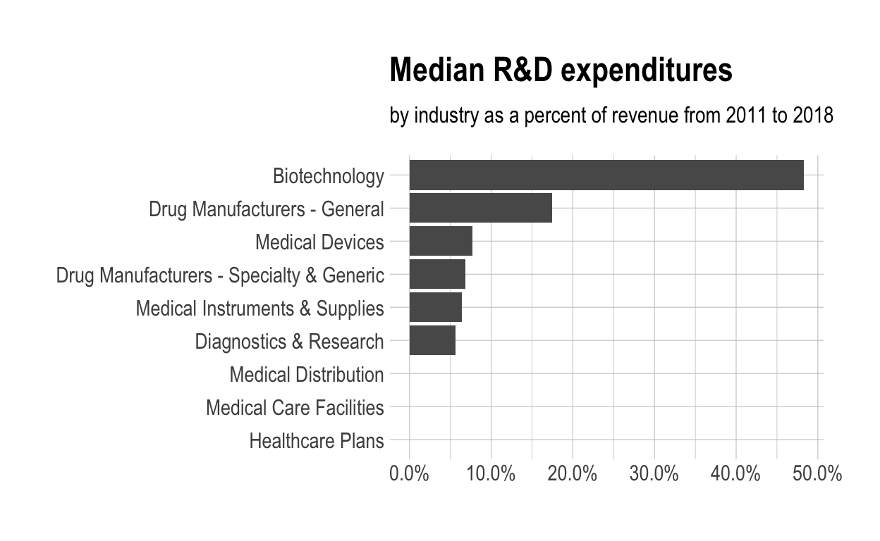
$ med_rnd_rev <dbl> 0.48317287, 0.05620271, 0.17451442, 0.06851879,…9.Create a static bar chart
-use ggplot to initialize the chart
-data is df
-the variable industry is mapped to the x-axis -reorder it based the value of med_rnd_rev
-the variable med_rnd_rev is mapped to the y-axis
-add a bar chart using geom_col
-use scale_y_continuous to label the y-axis with percent
-use coord_flip() to flip the coordinates
-use labs to add title, subtitle and remove x and y-axes
-use theme_ipsum() from the hrbrthemes package to improve the theme
ggplot(data = df,
       mapping = aes(
         x = reorder(industry, med_rnd_rev ),
         y = med_rnd_rev
         )) +
  geom_col() +
  scale_y_continuous(labels = scales::percent) +
  coord_flip() +
  labs(
    title = "Median R&D expenditures",
    subtitle = "by industry as a percent of revenue from 2011 to 2018",
    x = NULL, y = NULL) +
  theme_ipsum()
- Save the last plot to preview.png and add to the yaml chunk at the top
ggsave(filename = "preview.png",
       path = here::here("_posts", "2021-03-10-joining-data"))
11.Create an interactive bar chart using the package [echarts4r] (https://echarts4r.john-coene.com/index.html)
-start with the data df -use arrange to reorder med_rnd_rev -use e_charts to initialize a chart -the variable industry is mapped to the x-axis -add a bar chart using e_bar with the values of med_rnd_rev -use e_flip_coords() to flip the coordinates -use e_title to add the title and the subtitle -use e_legend to remove the legends -use e_x_axis to change format of labels on x-axis to percent -use e_y_axis to remove labels on y-axis- -use e_theme to change the theme. Find more themes here
df  %>%
  arrange(med_rnd_rev)  %>%
  e_charts(
    x = industry
    )  %>%
  e_bar(
    serie = med_rnd_rev,
    name = "median"
    )  %>%
  e_flip_coords()  %>%
  e_tooltip()  %>%
  e_title(
    text = "Median industry R&D expenditures",
    subtext = "by industry as a percent of revenue from 2011 to 2018",
    left = "center") %>%
  e_legend(FALSE) %>%
  e_x_axis(
    formatter = e_axis_formatter("percent", digits = 0)
    )  %>%
  e_y_axis(
    show = FALSE
  )  %>%
  e_theme("infographic")